Graphics
WulffPack offers several means to visualize the created particles. This page collects some examples.
Show a particle with matplotlib
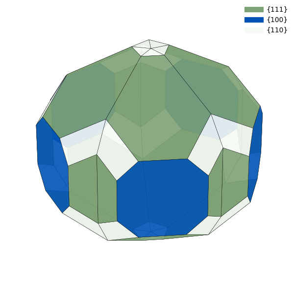
The simplest way to show a particle with WulffPack is with the
view function. The function uses
matplotlib and the user can specify colors of
facets, transparency and thickness of the lines between the facets via optional
keywords. The keyword save_as specifies the filename to save the figure as.
If none is specified, the particle is shown with the matplotlib GUI.
surface_energies = {(1, 1, 1): 1.0,
                    (1, 0, 0): 1.1,
                    (1, 1, 0): 1.12}
particle = Decahedron(surface_energies=surface_energies,
                      twin_energy=0.02)

# Define colors (optional)
colors = {(1, 1, 1): '#7da275',
          (1, 0, 0): '#0053b5',
          (1, 1, 0): '#f6faf5'}
# Show with GUI:
particle.view()
# Save as file:
particle.view(colors=colors, linewidth=0.3, alpha=0.9,
              save_as='single_particle.png')
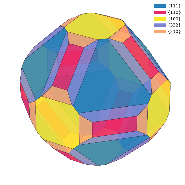
If the particle contains vicinal surfaces, it can be advantageous to
highlight the vicinality between surfaces with a continuous color scheme,
such that surfaces that are similar have similar colors.
WulffPack has a function
get_continuous_color_scheme, which creates
such color schemes automatically. Note that these color schemes are
sensible primarily for crystals with cubic symmetry.
surface_energies_vicinal = {(1, 1, 1): 1.0,
                            (1, 1, 0): 1.1,
                            (1, 0, 0): 1.1,
                            (3, 3, 2): 1.05,
                            (2, 1, 0): 1.15}
particle_vicinal = SingleCrystal(surface_energies_vicinal)
continuous_colors = particle_vicinal.get_continuous_color_scheme()
particle_vicinal.view(colors=continuous_colors)
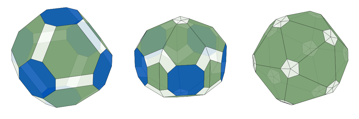
Make subplots
For more control over the matplotlib figure, one can also get axis objects directly. In the following snippet, a truncated octahedron, decahedron and icosahedron are created and put as subplots in the same figure.
Note that it can be quite tricky to get 1:1 aspect ratio when plotting 3D with
matplotlib. In this example, the figure size is manually set to three times as
wide as tall, and the distance from edge of the window to plot as well as
between plots is set to zero using subplots_adjust(). This ensures that the
plots are not squeezed in any direction.
import matplotlib.pyplot as plt

fig = plt.figure(figsize=(3 * 4.0, 4.0))
ax = fig.add_subplot(131, projection='3d')
particle = SingleCrystal(surface_energies)
particle.make_plot(ax, colors=colors)

ax = fig.add_subplot(132, projection='3d')
particle = Decahedron(surface_energies,
                      twin_energy=0.05)
particle.make_plot(ax, colors=colors)

ax = fig.add_subplot(133, projection='3d')
particle = Icosahedron(surface_energies,
                       twin_energy=0.05)
particle.make_plot(ax, colors=colors)

plt.subplots_adjust(top=1, bottom=0, left=0,
                    right=1, wspace=0, hspace=0)
plt.savefig('particles.png')
plt.show()
Visualize atoms objects
The possibility to extract an ASE Atoms object opens an arsenal of visualization opportunities. The arguably simplest one is ASE’s GUI.
from ase.visualize import view
view(particle.atoms)
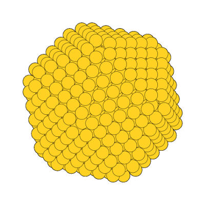
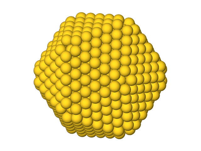
A truncated icosahedron visualized with ASE’s GUI.
Since an ASE Atoms object can be written to file, virtually any software that visualizes atomistic structures can be utilized.
from ase.io import write
write('atoms.xyz', particle.atoms)
Use wavefront .obj files
The write can write particles to
Wavefront .obj files.
Such files are useful in many 3D software, such as Blender.
particle.write('particle.obj')

A Winterbottom construction visualized
with Blender.
Source code
The complete source code is available in
examples/graphics.py
from wulffpack import (SingleCrystal,
                       Decahedron,
                       Icosahedron)

# Define energies and create particle
surface_energies = {(1, 1, 1): 1.0,
                    (1, 0, 0): 1.1,
                    (1, 1, 0): 1.12}
particle = Decahedron(surface_energies=surface_energies,
                      twin_energy=0.02)

# Define colors (optional)
colors = {(1, 1, 1): '#7da275',
          (1, 0, 0): '#0053b5',
          (1, 1, 0): '#f6faf5'}
# Show with GUI:
particle.view()
# Save as file:
particle.view(colors=colors, linewidth=0.3, alpha=0.9,
              save_as='single_particle.png')

# Use continuous color scheme
surface_energies_vicinal = {(1, 1, 1): 1.0,
                            (1, 1, 0): 1.1,
                            (1, 0, 0): 1.1,
                            (3, 3, 2): 1.05,
                            (2, 1, 0): 1.15}
particle_vicinal = SingleCrystal(surface_energies_vicinal)
continuous_colors = particle_vicinal.get_continuous_color_scheme()
particle_vicinal.view(colors=continuous_colors)

# Make figure with subplots
import matplotlib.pyplot as plt

fig = plt.figure(figsize=(3 * 4.0, 4.0))
ax = fig.add_subplot(131, projection='3d')
particle = SingleCrystal(surface_energies)
particle.make_plot(ax, colors=colors)

ax = fig.add_subplot(132, projection='3d')
particle = Decahedron(surface_energies,
                      twin_energy=0.05)
particle.make_plot(ax, colors=colors)

ax = fig.add_subplot(133, projection='3d')
particle = Icosahedron(surface_energies,
                       twin_energy=0.05)
particle.make_plot(ax, colors=colors)

plt.subplots_adjust(top=1, bottom=0, left=0,
                    right=1, wspace=0, hspace=0)
plt.savefig('particles.png')
plt.show()


# Use ase.visualize.view
from ase.visualize import view
view(particle.atoms)

# Write atoms to file for further visualization
from ase.io import write
write('atoms.xyz', particle.atoms)

# Write wavefront obj file
particle.write('particle.obj')